Embeddings in RAG: What They Decide Retrieval Can Find

Embeddings in RAG are fixed-length vectors that place chunk text and the user query in the same geometry so retrieval can rank passages by meaning rather than by shared keywords alone. At index time an embedding model turns each chunk into a vector and stores it in a vector database; at query time the same model embeds the question, and nearest-neighbour search returns the chunks whose vectors sit closest to that query vector under a similarity measure such as cosine similarity. Microsoft Learn’s Azure guide on the generate-embeddings phase states the rule that breaks indexes silently: the user query must be embedded with the same embedding model as the chunks, because swapping models compares incompatible spaces. That step sets the ceiling on what dense retrieval can find, which is why model choice, vector shape, domain fit and drift all sit under this hub rather than under the generator. Vector stores that hold those vectors include Weaviate, Pinecone, Qdrant and Milvus; store choice does not replace the embedding decisions that decide which neighbours exist. What follows defines embeddings, explains why they dominate recall, separates dense, sparse and multi-vector shapes, and routes each decision to the leaf that owns the mechanism.

What are embeddings in RAG?

Embeddings in RAG are numeric vectors produced by an embedding model from text (and sometimes images or other modalities) so that items with similar meaning land near each other in vector space. Telerik’s “What Are RAG Embeddings?” frames the job as capturing meaning so a search system can compare meaning rather than only matching strings. IBM’s RAG cookbook overview of embeddings treats the same object as the bridge between language and nearest-neighbour search: once both the corpus and the query are points, retrieval becomes a geometry problem. Galileo’s selection guide opens the same way: an embedding is a numerical representation of text that makes semantic comparison computable.

In a retrieval-augmented generation pipeline the embedding step runs twice with the same model. Microsoft Learn’s Azure generate-embeddings phase places the first pass after chunking, when each chunk is embedded and written into the vector index, and the second pass at query time, when the user question is embedded before search. Medium’s production guide from Sharan Harsoor walks the same path through tokenization into vectors: the model does not store the original string as the retrieval key; it stores a fixed-dimensional list of floating-point numbers. Cosine similarity on normalised vectors is the usual distance for dense retrieval, though dot product and Euclidean distance appear depending on how the store indexes the space.

Dense single-vector embeddings are the default shape for most RAG indexes because one vector per chunk is cheap to store and fast to compare. Learned sparse embeddings sit beside them when exact tokens still matter more than paraphrase. Multi-vector late interaction is a different retrieval shape entirely: many vectors per document instead of one. The field of decisions that follow from that definition is large enough that the next question is not “what is a vector” but why two incompatible embedding models destroy retrieval even when both models look strong on a public board.

Why must the same embedding model run at index time and query time?

The same embedding model must run at index time and query time because dense retrieval ranks by distance inside one learned space, and a different model defines a different space even when both models share a dimension count. Microsoft Learn states the operational rule directly for Azure RAG: embed the user query with the same embedding model as your chunks, then search for the most semantically relevant vectors. If yesterday’s chunks were embedded with model A and today’s queries are embedded with model B, cosine neighbours are comparing apples to oranges and recall collapses without a loud error.

That constraint is why embedding upgrades are migrations rather than config flips. Replacing the model means re-embedding the corpus, rewriting the vectors in the store, and only then serving queries from the new space. Weaviate, Pinecone, Qdrant and Milvus can all hold the new vectors, but none of them can mix two incompatible spaces into one meaningful ranking. The sibling mechanism for measuring when indexed and query distributions have already diverged is detecting embedding drift; the failure symptom when quality slides without a deliberate model change is retrieval quality degradation.

Teams sometimes try to dodge the cost by keeping old vectors and only embedding new documents with a newer model. That creates a mixed-time index: two geometries in one collection. Azure’s generate-embeddings guidance and Galileo’s selection framing both treat model identity as part of the retrieval contract, not as an interchangeable API detail. Once that contract is clear, the deeper question is why the embedding step, not the language model, decides what can appear in the prompt at all.

Why do embeddings decide what retrieval can find?

Embeddings decide what retrieval can find because every dense candidate is ranked only by how close its vector sits to the query vector, so anything the model cannot represent well cannot surface in the top-k. Microsoft Learn’s Azure generate-embeddings phase opens with that importance claim: the embedding model you choose can significantly affect the relevancy of vector search results. Galileo’s “Mastering RAG: How to Select an Embedding Model” makes the same point from the evaluation side: embeddings sit on the critical path for question answering, conversational search and tool fetching because bad neighbours starve the generator of evidence.

Vocabulary is the first structural limit. Azure notes that every embedding model is trained with a specific vocabulary; BERT-scale vocabularies sit around 30,000 words in the example they cite. When a domain word is missing, many models split it into subwords. Azure’s histamine example shows the damage: histamine may become his, ta and mine, whose meanings diverge from the chemical, so the resulting vector matches poorly even when the document is relevant. IBM’s performance-versus-cost framing and Google Cloud’s RAG Engine embedding notes both treat model fit to the corpus as a first-order choice rather than a cosmetic one.

Cost and capacity are the second limit. Larger vectors usually score better on public suites but cost more storage and compare time; smaller vectors are cheaper. Azure’s dimensionality-reduction section and Galileo’s vector-dimension discussion both warn that public leaderboards often sit on academic datasets that may not match your corpus, so the defensible move is to measure recall on labelled queries from your own traffic. When the geometry is wrong, the failure shows up as retrieval, not as a “bad LLM”: user words that never match document words are vocabulary mismatch; a returned passage that does not contain the answer is wrong-chunk retrieval. How close two vectors are scored is its own decision on cosine, dot product and Euclidean. How much dimension you keep lives on embedding dimensions.

How do dense, sparse and multi-vector embeddings differ for RAG?

Dense, sparse and multi-vector embeddings differ by what each dimension means and how many vectors stand for one document. A dense embedding is a short vector of real numbers, typically hundreds to a few thousand dimensions, where every coordinate is usually non-zero and meaning is distributed across the whole vector. That is the default RAG path in Azure, IBM, Galileo and the Medium production walkthroughs that define embeddings for retrieval: one vector per chunk, nearest neighbours by cosine or equivalent.

A sparse embedding is a high-dimensional vector over vocabulary-sized coordinates where most values are zero and the non-zero weights highlight terms the model treats as important. Learned sparse methods such as SPLADE sit between classic BM25 and dense vectors: they keep exact-term behaviour while learning which expansions help. Weaviate’s hybrid search documentation describes combining vector search with BM25 keyword search so semantic similarity and exact keyword relevance both influence the ranking, with a server-side alpha default of 0.75 toward vectors when alpha is left unset (as of September 2026). The depth for when learned sparse beats dense alone is SPLADE and learned sparse retrieval; the depth for BM25 itself is BM25.

Multi-vector and multimodal shapes change the unit again. Azure’s generate-embeddings phase includes a multimodal branch: embed images and text into a shared space, or preprocess multimodal content before indexing. Milvus’s 2026 embedding-model comparison adds cross-modal retrieval as a first-class test, not a footnote. One vector per image-plus-caption pair is still dense retrieval; late-interaction multi-vector models keep many vectors per document and score interactions at query time. Those designs cost more at search time and need different evaluation. Native multimodal embedding depth lives on embedding images and text together. Once the shape family is clear, the practical question is which decision to make first on a real corpus.

Which embedding decision should you make next?

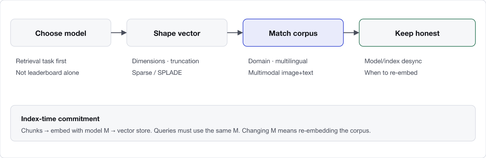
The next embedding decision is the one your measurements force, not the one a public leaderboard highlights. A defensible starting path on the pages that dominate this topic (Azure’s choose-an-embedding-model flow, Galileo’s selection framing, Milvus’s bake-off caution that MTEB alone is not enough) is: pick a strong general retrieval model, measure recall on your labelled queries, and graduate to domain, language, modality or sparse upgrades only when the metrics justify the ingest cost. How to choose an embedding model owns that procedure; the family catalogue behind vendor names sits under embedding model families.

Vector shape comes next when storage, latency or exact-term miss rates dominate. Shrinking vectors, Matryoshka truncation and mismatch failures belong on embedding dimensions, truncation and Matryoshka. Exact identifiers that dense neighbours keep missing belong on when to use sparse embeddings and often on hybrid search. Corpus fit comes after the general model is honest: domain vocabulary that subwords destroy belongs on fine-tuning embeddings for your domain; cross-language questions belong on multilingual RAG; image and text in one index belong on multimodal embeddings.

Keep the index honest after ship. When quality falls with no deliberate model change, measure whether indexed and query distributions diverged on when to re-embed after drift before you blame the generator. Building the first end-to-end path that embeds chunks into a store and retrieves them for a prompt is the job of how to build a RAG pipeline. The hub’s job stops at naming the decision; each leaf owns the mechanism, the costs and the failure modes.

Embeddings turn chunks and queries into vectors so retrieval can rank by meaning, and that single step sets the ceiling on what dense RAG can find. Microsoft Learn, Galileo, Telerik, IBM and the production Medium guides on this topic agree on the mechanics: same model at index and query time, vocabulary that must cover the corpus, and evaluation on your own labelled queries rather than on a leaderboard alone. Dense vectors are the default; sparse and multimodal shapes exist for exact terms and mixed media. Choose the model, shape the vector, fit the corpus, then watch for drift. The leaves under this hub own each of those decisions in depth so the next change matches the measurement that forced it.