Indexing for RAG: Structures, Trade-offs and Limits
What the index does to recall, latency and memory. Flat, HNSW, IVF, quantization, filters, tenants and updates.
Indexing for RAG is the structure that stores chunk embeddings so approximate nearest-neighbour search can return candidates without scanning every vector, and the structure you pick sets the recall, latency and memory ceiling. IBM’s vector-database overview for RAG, Machine Learning Mastery’s indexing-strategies chapter, MyScale’s vector-indexing guide, AI Bites’ seven-method survey, Writer’s RAG vector-database explainer, YugabyteDB’s vector-indexing primer, Meilisearch’s RAG indexing guide, Towards AI’s millisecond-retrieval piece and ZenML’s vector-database roundup (all extracted September 2026) treat the index as the layer that turns embeddings into searchable neighbours. This hub defines that job, names the three dials the index controls, and routes depth to the six children that own HNSW, IVF and flat indexes, quantization, metadata filtering, multi-tenancy and updates.
What is indexing in RAG?
Indexing in RAG is the step that turns already-embedded chunks into a searchable structure such as a flat scan, an HNSW graph or an IVF partition set so a query embedding can find near neighbours without comparing every stored vector. Meilisearch’s RAG indexing guide states that indexing organises data so the retriever locates relevant text without scanning the whole knowledge base. Machine Learning Mastery (Palomares) frames indexing strategies as the way similarity search stays fast while trading measured accuracy. Weaviate’s vector-index concepts page (as of September 2026) defines a vector index as the data structure that organises embeddings for efficient similarity search and lists HNSW, flat and dynamic indexes as first-class options.
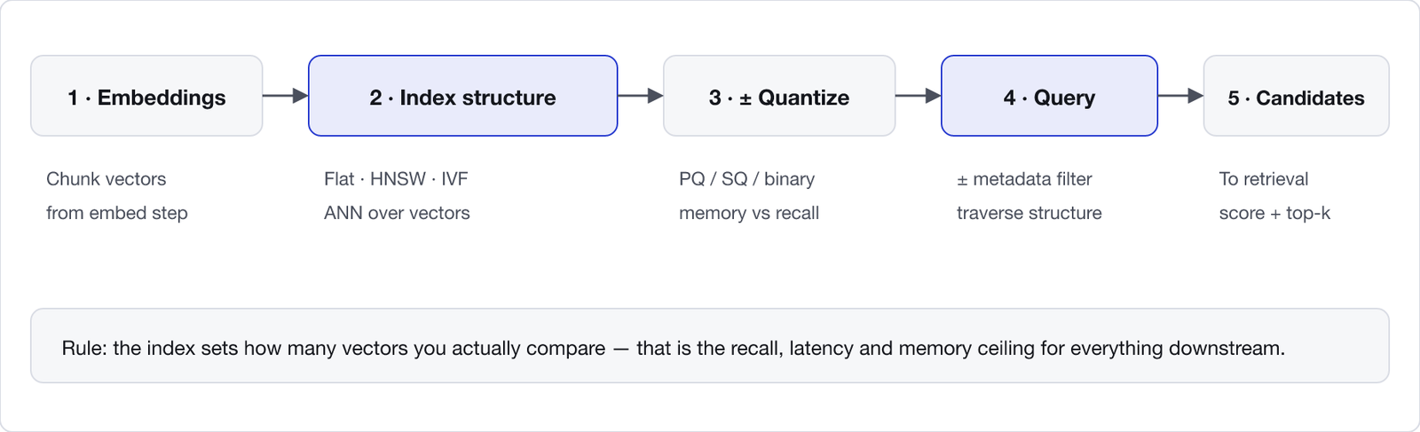
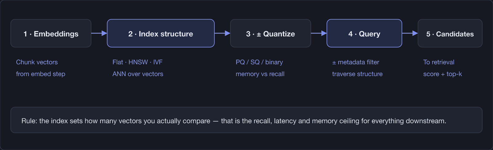
The lean build path is the same across those sources. Chunks are embedded first under embeddings. An approximate nearest-neighbour structure is built over those vectors. Optional quantization shrinks memory. At query time the structure is traversed, metadata filters are applied when present, and candidates return to retrieval. Document splitting is not indexing: how units are cut lives under chunking. Hybrid BM25-plus-vector scoring is retrieval, not an index type, and lives under hybrid retrieval.
Weaviate’s documentation (as of September 2026) notes that HNSW is a custom CRUD-capable implementation of Hierarchical Navigable Small World graphs, that a flat index stores every vector in one list for small collections, and that a dynamic index can start flat and switch to HNSW past a scale threshold. Those three options are the production defaults this hub routes. Secondary algorithms such as LSH or Annoy appear in survey pages such as AI Bites; they are not mapped children on this site.
Once the stage is clear, the next question is why picking the wrong structure shows up as a wrong answer rather than as a slow dashboard.
Why does the index choice change recall and latency?
The index choice changes recall and latency because every approximate structure trades how many vectors it actually compares for how much memory and build cost it spends. Flat search is exact and linear in corpus size. HNSW pays RAM for a multi-layer graph that usually keeps recall high under continuous inserts. IVF scans only a subset of clusters and needs rebuild discipline when the data distribution moves. Machine Learning Mastery and MyScale both open on that trade-off rather than on a single “best index” claim.
Milvus IVF-versus-HNSW guidance in the live teardown set reports that without compression IVF recall can reach the mid-90s percent range while HNSW usually sits higher, and that under heavy metadata filtering HNSW graph traversal can degrade while IVF stays more stable via centroid-level coarse filters. Those bands are vendor-reported for their own benchmarks; verify on your corpus before you treat them as SLAs. BigData Boutique’s Syn-Hershko write-up (29 May 2026), cited across prior indexing teardowns and echoed in this session’s structure pages, reports HNSW memory overhead roughly 2 to 5 times raw vectors versus IVFFlat near 1.1 times, and notes that HNSW absorbs inserts without a full rebuild while IVFFlat recall drifts as data changes. Writer and YugabyteDB primers make the same qualitative point: the index is a budget, not a free speedup.
Wrong neighbours become wrong RAG answers because the generator answers the context it receives. Indexing errors bubble into retrieval misses that look like generation faults, a sequencing rule Weaviate’s RAG evaluation writing has stated elsewhere on this site. Measuring hit rate before you change the prompt is how you keep the fault on the right leaf. Depth on graph parameters lives on how HNSW is built and searched; depth on clusters lives on IVF and flat indexes; depth on compression lives on cutting vector memory.
What index structures does RAG actually use?
Production RAG indexes cluster into three structures and one memory dial. Flat indexes scan every vector and win only while the collection stays small. HNSW indexes build hierarchical navigable small-world graphs and are the default for high-recall serving when RAM allows. IVF indexes partition the space into clusters and probe a subset at query time. Quantization compresses vectors so more of the graph or cluster set fits in memory. AI Bites lists additional methods; IBM, Towards AI and ZenML keep the practical shortlist closer to HNSW, IVF and flat with compression as an add-on.
Weaviate’s concepts page (as of September 2026) matches that shortlist: HNSW for logarithmic query scaling, flat for small datasets, dynamic for automatic flat-to-HNSW switching, and quantization pages for product, binary and scalar compression. The leaf for graph build and ef / maxConnections trade-offs is HNSW explained. The leaf for nlist / nprobe and exact scan is IVF, flat and the recall you trade for speed. The leaf for PQ, BQ and SQ is quantization.
Stores that ship those structures include Weaviate, Pinecone, Qdrant and Milvus. Naming a store is not choosing an index: the same product can expose more than one structure, and the wrong structure inside a strong store still returns the wrong neighbours. Meilisearch and ZenML both warn against treating the database brand as a substitute for an index decision.
What production constraints does the index have to survive?
Production constraints are the reasons an index that looked fine on a static demo fails after users, tenants and deletes arrive. Metadata filtering changes which neighbours are legal. Multi-tenancy isolates shards so one customer never reads another customer’s vectors. Updates and deletes keep the graph or cluster set honest when source documents move. Meilisearch’s RAG indexing guide treats refresh and evaluation as part of indexing work. Writer and IBM both stress that the serving path must respect permissions and freshness, not only cosine distance.
Filtered search depth lives on metadata filtering in vector search, including pre-filter and post-filter behaviour and the recall collapse that follows a too-tight predicate on a sparse graph. Tenant isolation depth lives on multi-tenancy and isolation, with the failure symptom on when RAG returns another tenant’s documents. Mutate mechanics live on updating and deleting documents in a vector index, with the freshness failure on stale index. Change detection that decides when to call those APIs lives on incremental indexing.
Weaviate’s multi-tenancy documentation (as of September 2026) states that each tenant is stored on a separate shard and that data in one tenant is not visible to another. Its update documentation states that partial updates use PATCH, complete replacements use PUT, and updates that include vectorised text properties recalculate embeddings and reindex. Those product facts belong on the leaves; the hub only needs the rule that production constraints are index concerns, not prompt concerns.
How do you choose between HNSW, IVF and flat for RAG?
You choose between HNSW, IVF and flat by matching write pattern, memory budget and filter load to the structure’s failure mode, then measuring recall on your own queries. HNSW is the usual default when RAM allows and documents keep arriving, because inserts update the graph without a full rebuild. IVF is the usual default when memory is tight or when heavy metadata filters make cluster-level coarse filtering more stable. Flat is the usual default only while the collection is small enough that a full scan still meets latency.
Milvus and BigData Boutique both frame that decision as a measured trade-off rather than as a brand preference. Weaviate’s dynamic index (as of September 2026) automates one common path: start flat, switch to HNSW past a threshold. That automation does not remove the need to measure filtered recall after the switch. AI Bites and MyScale list more exotic ANN families; leave those until Flat, HNSW and IVF have failed a measured test on your corpus.
If the decision is really about compression, open the compression leaf before you abandon HNSW. If the decision is really about permissions, open filtering and multi-tenancy before you rebuild clusters. If the decision is really about stale answers, open updates and incremental ingest before you retune ef.
IBM’s RAG vector-database overview and ZenML’s roundup both remind practitioners that the store and the index are related but not identical decisions. A managed service can hide HNSW parameters behind defaults and still leave you with the wrong neighbour set if filters, tenants or deletes were never designed. Towards AI’s millisecond-retrieval framing and YugabyteDB’s primer make the latency side vivid; Meilisearch and Machine Learning Mastery make the organisation side vivid. Put together, the live ranking set demands a map that separates structure choice from production constraint choice.
A practical measurement order keeps the hub honest. Confirm the collection size and write rate. Confirm whether queries carry metadata predicates and how selective those predicates are. Confirm whether tenants share a process or require shard isolation. Confirm whether deletes are required for compliance. Only then pick Flat, HNSW or IVF and decide whether quantization is mandatory. Skipping that order is how teams rebuild graphs for a permissions bug or add compression for a missing delete path.
Secondary ANN families such as locality-sensitive hashing appear in AI Bites and similar surveys. They stay outside this hub’s children because production depth on this site concentrates on Flat, HNSW, IVF, quantization, filtering, multi-tenancy and updates. If a measured experiment shows those six cannot meet a latency or memory bar, document the experiment and reopen the map; do not silently redefine indexing as chunking or as hybrid retrieval.
ZenML’s vector-database roundup and IBM’s RAG store overview both surface a second failure mode: teams compare product feature matrices before they compare index structures. Feature matrices matter for operations, but they do not answer whether your filtered queries keep recall when 90 percent of candidates are excluded, or whether deletes leave tombstones that still retrieve. Those questions are index questions. Answer them on the leaves, then pick a store that can run the structure you measured.
Meilisearch’s RAG indexing guide also lists hierarchical and multi-representation document strategies under indexing language. On this site those strategies belong with chunking and parent-document retrieval, not with ANN structures. Keeping that border prevents the hub from becoming another mega-guide that teaches chunk size under an indexing title. The same border applies to GraphRAG: relationship graphs are architecture material, not a substitute for HNSW or IVF.
Where should you go next from this indexing hub?
Start with HNSW if you need the default graph index and its parameters. Start with IVF and flat if memory, rebuild windows or filter stability dominate. Start with vector quantization if RAM is the bottleneck. Start with metadata filtering if legal neighbours are a subset of geometric neighbours. Start with multi-tenancy if isolation is the product requirement. Start with updates and deletes if removed documents still answer.
Machine Learning Mastery, Meilisearch, IBM, Writer, YugabyteDB, Towards AI, ZenML, AI Bites and MyScale all describe pieces of that map. None of them is both a lean stage hub and a full router to the six production leaves this site needs. The gain here is that separation: structures on one side, production constraints on the other, with every union topic either present or explicitly owned elsewhere.
Indexing is finished for a collection when the structure matches the write and filter load, memory fits the budget, deletes actually remove vectors, and measured recall on filtered queries meets the bar you set. Everything before that is still an index decision. Everything after that is retrieval and generation over whatever neighbours the index returned. Pick the structure deliberately, measure it under your filters, and open the leaf that owns the dial you are about to turn.
Across the nine live extracts for this rebuild, the shared demand is a clear account of how embeddings become neighbours and which dials move recall, latency and memory. IBM, Machine Learning Mastery, MyScale, AI Bites, Writer, YugabyteDB, Meilisearch, Towards AI and ZenML each carry pieces of that account. This hub takes the union, separates structures from production constraints, and routes every remaining depth question to a named child so the reader is never left with an editorial label where a mechanism page should be.
When the structure, the filters, the tenants and the delete path all match the workload, indexing stops being the mystery stage of RAG and becomes a measured budget. Turn the dial that owns the miss, then re-measure. That is the whole job of this hub.
Use the structure leaves when neighbours are wrong geometrically. Use the production leaves when neighbours are wrong legally, organisationally or temporally. Keep that split and the index stops being a black box.
Measure recall under your filters twice before you rebuild the index once.